The Volatility Tax: Why Consistent Models Earn More
Steady Numerai models earn far more cumulative NMR than volatile peers with the same mean MMC — burns and compounding turn score variance into a tax.
Within the high-skill tercile of 9,100+ staked models, the steadiest 20% earned roughly 5x the cumulative NMR of the most volatile 20% — same average MMC, very different outcomes. Numerai's payout mechanics make inconsistency expensive. Two models with identical average MMC (Meta Model Contribution) can produce very different cumulative returns depending on how much their scores swing round to round. Steadier models tend to keep more of their gains after burn rounds and stake-base compounding.
This article quantifies the volatility tax using tournament data, explains the mechanics behind it, and shows the penalty holds after controlling for skill level. For background on scoring, see How Numerai Works.
The Payout Formula and Compounding
Each round, a model's payout is:
payout = stake x clip(0.5 x CORJ60 + 2.0 x MMC, -0.25, 0.25) x payout_factor
The clip function caps the combined score between -0.25 and +0.25. A model scoring 0.30 is paid as if it scored 0.25, and a model scoring -0.30 is burned as if it scored -0.25. The cap is symmetric, but cumulative staking returns are not just an arithmetic average of scores. Burn rounds reduce the stake base that future positive rounds compound from.
In practice, the caps rarely bind. Most raw scores fall well within the range.
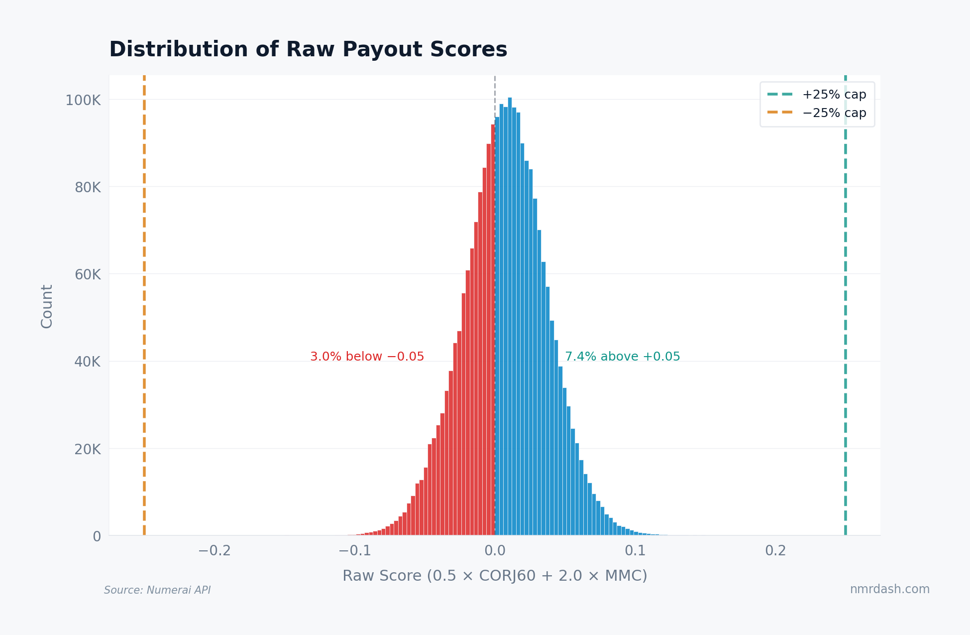
The distribution clusters near zero: 7.4% of observations score above +0.05, and 3.0% fall below -0.05. The +/-0.25 caps sit far out in the tails. Clipping is not the main story in most rounds; variance drag on cumulative returns is.
Where the Tax Actually Bites
Even without hitting the caps, volatile scores compound poorly. A model alternating between +0.03 and -0.02 averages +0.005 per round — the same as a model that scores +0.005 every round. But the volatile model's burn rounds eat into the stake base, so each subsequent positive round is worth less in absolute NMR. Over hundreds of rounds, that drag accumulates.
Plotting MMC volatility against cumulative payout across 9,100+ staked models (each with 50+ rounds) makes the effect visible.
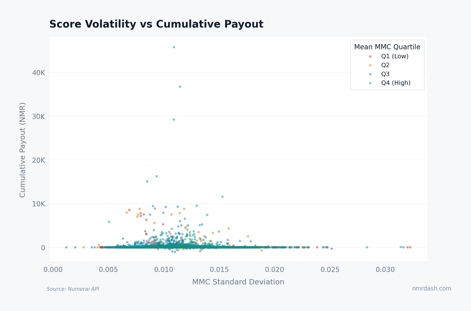
The largest cumulative payouts sit in the lower half of the volatility range, and above roughly 0.017 standard deviation the big earners disappear entirely. Some high-volatility Q4 (high mean MMC) models do accumulate positive payouts, but big returns skew heavily toward steadier performers. Negative outliers span the full volatility range but tilt right.
The correlation between MMC standard deviation and cumulative payout is -0.045. That sounds small, but the scatter shows a nonlinear pattern the coefficient misses. Volatility imposes a floor more than a ceiling: steady models are not guaranteed to earn, but volatile models face a structural headwind. You can explore individual model histories on the Models page.
Controlling for Skill
An obvious counterargument: maybe volatile models just have worse average MMC. To test whether the penalty persists after controlling for skill, we split models into mean-MMC terciles (low, mid, high) and then into volatility quintiles (Q1 = steadiest, Q5 = most volatile) within each tercile.
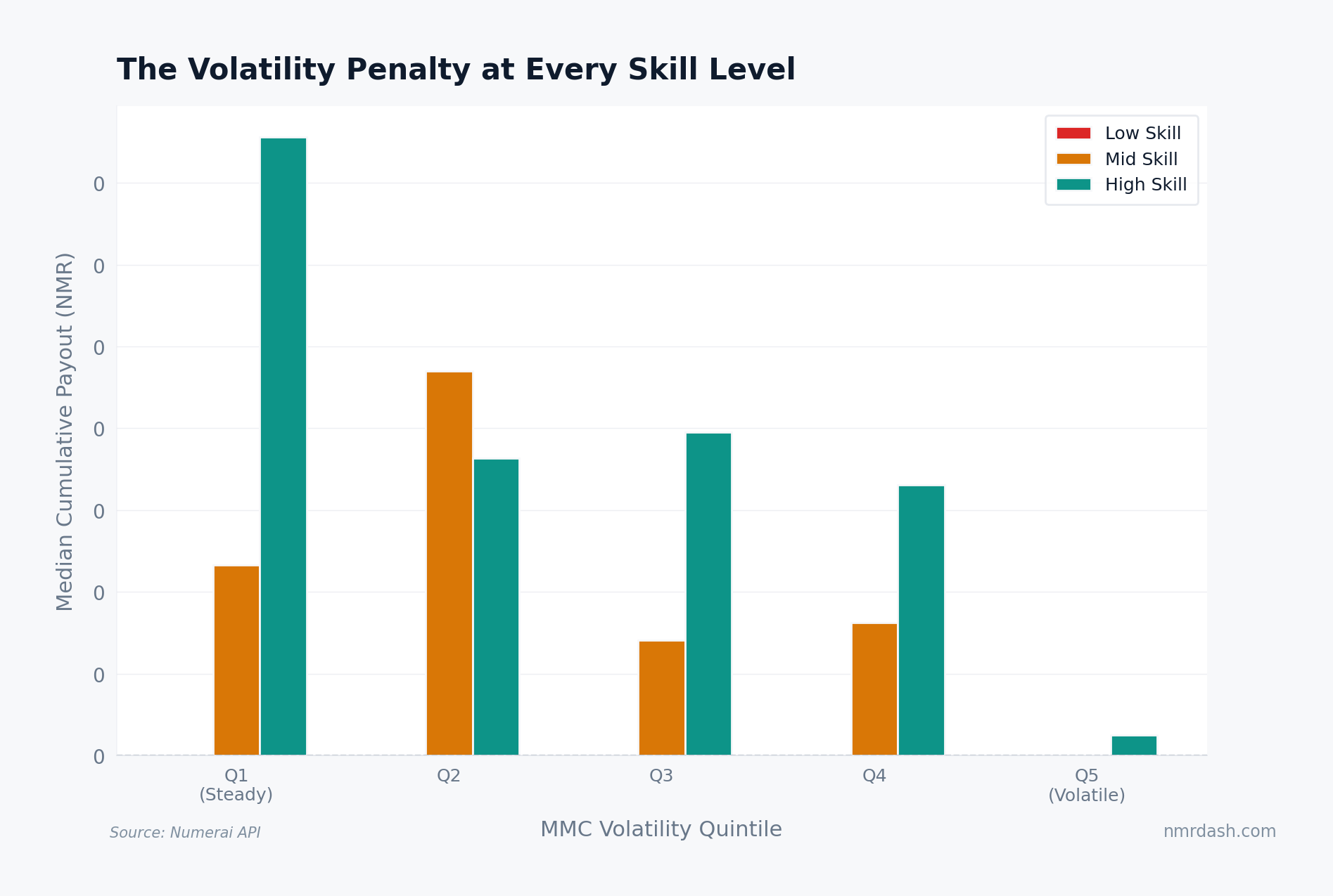
The pattern holds at every skill level. Within the high-skill tercile, steady models (Q1) earn a median cumulative payout roughly 5x that of the most volatile (Q5). Mid-skill shows the same direction — its most volatile quintile earns close to nothing. Low-skill models earn little regardless of volatility — consistency cannot compensate for a weak signal.
Mean payouts reinforce this. High-skill Q1 averages 143.6 NMR per model; high-skill Q5 averages 91.5 NMR. The penalty scales with stake size, because larger stakers compound more aggressively in both directions.
A Simulation of the Mechanism
To isolate the mechanics, consider three simulated models over 500 rounds. "Steady" has mean MMC 0.010, standard deviation 0.005. "Moderate" has mean 0.012, standard deviation 0.015. "Volatile" has the highest raw skill (mean 0.015) but standard deviation 0.025. All use the same payout formula with clipping applied.
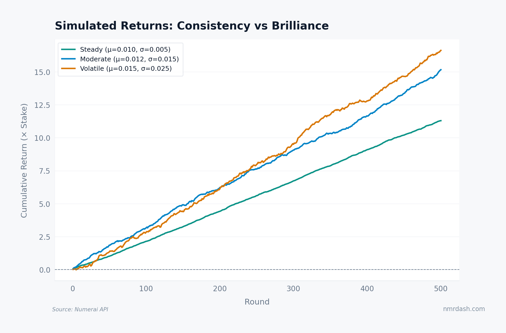
The result is a useful negative control: the volatile model finishes ahead. Tournament-scale scores sit so far inside the ±0.25 caps that clipping almost never binds, and a 50% edge in mean skill dominates a simple sum of scores. The payout formula alone does not tax volatility. The tax appears when mean skill is held equal — the situation the quintile comparison above measures — and through the stake base itself: real burn rounds remove NMR that later wins can no longer compound, an effect a raw score sum understates.
Why This Matters for Stakers
The volatility tax has direct implications for anyone staking NMR.
- Model selection: At the same average MMC, the lower-volatility model keeps more of its gains over a year of rounds. Prioritize consistency alongside peak scores.
- Stake sizing: The penalty compounds with stake size. Larger stakers should weight consistency more heavily, because burn rounds remove more absolute NMR from the compounding base.
- Ensemble strategies: Running multiple models with moderate skill but low correlation reduces portfolio-level volatility. The diversification paradox explores this tradeoff.
- The payout factor changes the scale: The factor multiplies both gains and burns. When it is low, absolute payout per round shrinks, so recovery from prior burns is slower in NMR terms; when it is high, both good and bad rounds matter more.
In practice the tournament rewards models that are reliably decent over models that are occasionally brilliant. Variance is not free. Building for consistency (lower drawdowns, stable signal) is not just risk management. It is an expected-value optimization.